Advanced analytics and inference
By the end of this module you will be able to:
- Classify machine learning problems and explain overfitting and cross-validation
- Apply feature engineering principles to improve model performance
- Distinguish stream processing from batch processing and identify the right approach for time-sensitive workloads
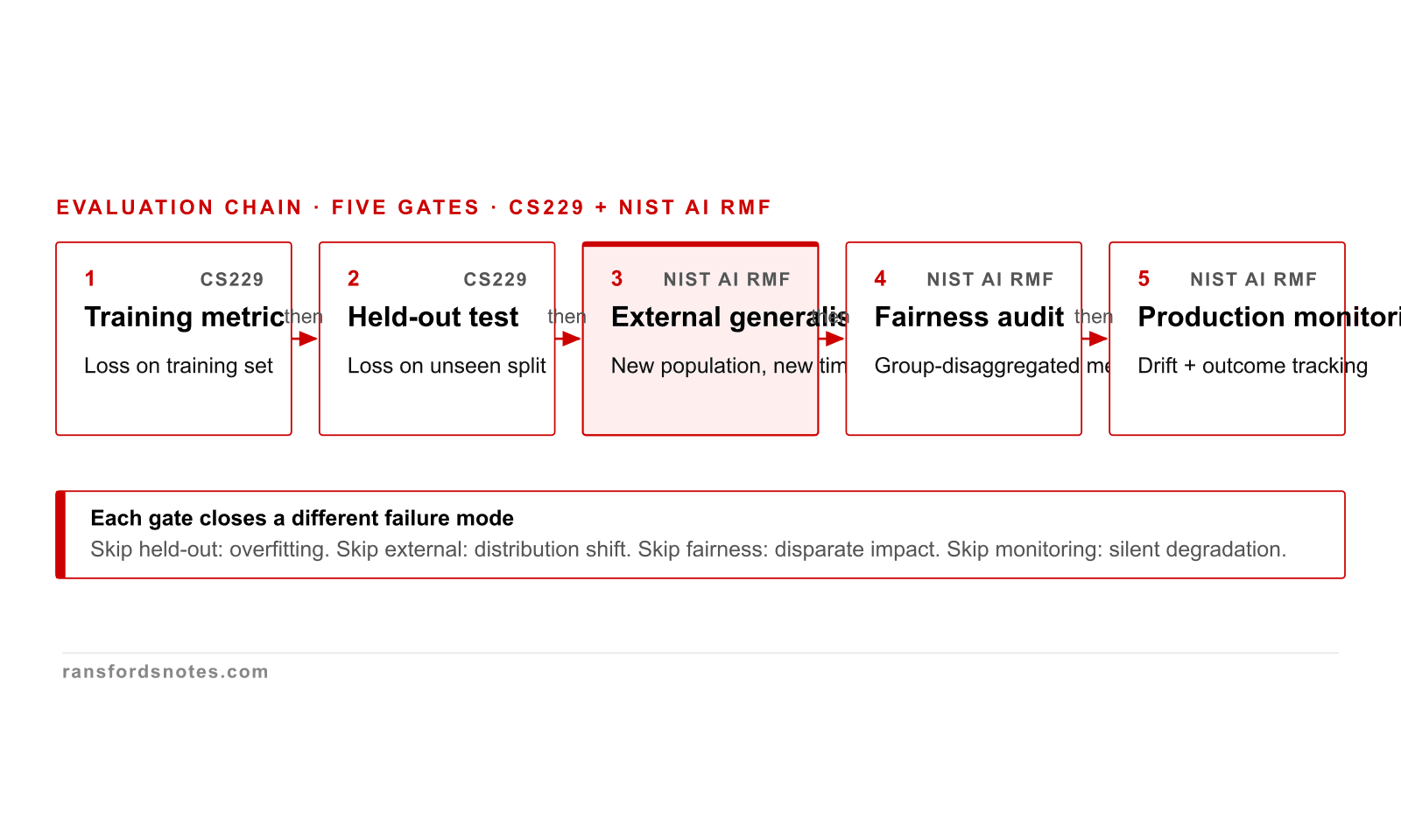
Advanced analytics evaluation chain has five named gates
Advanced analytics evaluation has five gates from training metric through fairness audit to production monitoring.
An advanced analytics evaluation chain has five gates: training metric, held-out test, external generalisation, fairness audit, production monitoring. Each gate closes a different failure mode. NIST AI RMF 1.0 Measure function names all five as mandatory before deployment.
Four non-causal explanations every correlation must rule out
Correlation has four common non-causal explanations: confounding, reverse causation, selection bias, chance.
Correlation has four common non-causal explanations: confounding (common cause), reverse causation, selection bias, and chance. Hill 1965 named nine criteria for inferring causation from observational data; Pearl 2009 formalised the framework with directed acyclic graphs.
Real-world failure · 2016
Microsoft Tay: a language model that overfit to adversarial inputs within 16 hours
In March 2016, Microsoft deployed Tay, a conversational AI trained on social media conversations, with the intention of it learning from interactions with Twitter users. Within 16 hours, coordinated groups of users had fed Tay a continuous stream of offensive content. The model learned from these interactions in real time, producing increasingly harmful outputs. Microsoft took Tay offline after less than a day.
The failure illustrates a fundamental challenge in machine learning: a model trained on a sample of the data distribution may behave unpredictably on inputs that fall outside that distribution (out-of-distribution inputs), particularly adversarial inputs deliberately designed to exploit the model. Tay had no mechanism to detect that the inputs it was receiving differed systematically from its training distribution.
The incident accelerated the development of adversarial robustness as a research area and contributed to the safety evaluation frameworks now standard in large language model deployment. Every model deployed to real users encounters a noisier, more adversarial distribution than its training set. Measuring this gap is part of responsible ML deployment.
Tay was trained on public Twitter conversations. Its training process had no safeguards against adversarial examples. What does this teach about the difference between in-distribution and out-of-distribution inputs?
With the learning outcomes established, this module begins by examining machine learning taxonomy in depth.
23.1 Machine learning taxonomy
Machine learning problems are classified by the structure of the learning signal. Supervised learning uses labelled examples: each training example pairs an input with the correct output. Classification (predicting a discrete label) and regression (predicting a continuous value) are both supervised. Examples include spam detection, image classification, and house price prediction.
Unsupervised learning finds structure in unlabelled data. Clustering (k-means, DBSCAN, hierarchical clustering) groups similar examples. Dimensionality reduction (PCA, UMAP, t-SNE) compresses high-dimensional data to lower dimensions for visualisation or downstream processing. Anomaly detection identifies points that differ from the learned distribution.
Reinforcement learning trains an agent to take actions in an environment to maximise a cumulative reward signal. It requires no pre-labelled dataset but requires a defined reward function and either a simulation or a real environment. Applications include game playing (AlphaGo), robot control, and recommendation system optimisation where explicit labels are unavailable.
Self-supervised learning (the technique underlying transformer language models) creates labels from the data itself. BERT masks tokens and trains the model to predict them. GPT-style models train on next-token prediction. The label is derived from the input, which makes it possible to train on the entire web without manual annotation.
With an understanding of machine learning taxonomy in place, the discussion can now turn to overfitting, underfitting, and cross-validation, which builds directly on these foundations.
“All models are wrong, but some are useful. The question is: how wrong do they have to be to not be useful?”
George Box, paraphrased from 'Robustness in the Strategy of Scientific Model Building' (1979)
Box's aphorism is a reminder that the goal of a model is not to perfectly represent reality but to provide useful approximations for specific decisions. A weather forecast model that is accurate to within 2 degrees is useful for planning outdoor events even if it is not physically correct in every detail. Practitioners should ask 'what decisions does this model support?' before evaluating whether it is accurate enough.
“All models are wrong, but some are useful.”
George E. P. Box, Journal of the American Statistical Association (1976) - Science and Statistics
Box's aphorism remains the most important sentence in applied statistics. It reframes the question from 'Is the model correct?' to 'Is the model useful enough for the decision at hand?'
23.2 Overfitting, underfitting, and cross-validation
Overfitting occurs when a model learns the training data too well, including its noise and idiosyncrasies, and fails to generalise to new data. A decision tree with no depth limit will perfectly classify all training examples by memorising them, but will perform no better than chance on unseen data. High training accuracy with poor validation accuracy is the diagnostic signal.
Underfitting occurs when a model is too simple to capture the underlying structure of the data. A linear model applied to data with clear nonlinear relationships will underfit: both training and validation accuracy will be poor. The bias-variance trade-off describes this tension: high-bias (simple) models underfit; high-variance (complex) models overfit.
k-fold cross-validation addresses the problem of having too little data for a proper train/validation/test split. The dataset is divided into k folds. The model is trained k times, each time using k-1 folds for training and the held-out fold for validation. The k validation scores are averaged to estimate generalisation performance. Five-fold and ten-fold cross-validation are standard in practice.
Feature engineering transforms raw data into representations that make the underlying patterns more accessible to the model. Temporal features (day of week, hour of day, days since last purchase) extracted from timestamps often improve performance more than adding new raw features. Interaction terms (product of two features) capture non-additive effects. Scaling (standardisation, normalisation) is required for distance-based algorithms and gradient-based optimisation.
With an understanding of overfitting, underfitting, and cross-validation in place, the discussion can now turn to stream processing and time-sensitive analytics, which builds directly on these foundations.
Common misconception
“More data always improves model performance.”
More data helps when the model is underfitting due to insufficient training examples. But additional data does not fix: a model applied to the wrong problem (wrong features), a model with a fundamental architecture mismatch, label noise in the training data, or distribution shift between training and deployment environments. The quality and representativeness of data matters more than quantity. A model trained on 10 million biased examples will be more confidently wrong than one trained on 100,000 balanced examples.
Common misconception
“Deep learning always outperforms traditional statistical methods.”
For structured tabular data with thousands of rows, gradient-boosted trees consistently match or outperform deep learning. Neural networks excel at unstructured data (images, text, audio) where feature engineering is impractical. The 2022 Kaggle survey showed XGBoost as the most-used algorithm for tabular competitions, ahead of any deep learning approach.
23.3 Stream processing and time-sensitive analytics
Batch processing computes analytics over a fixed dataset: all the data from yesterday is processed in a single job that runs each night. Latency is acceptable (hours or overnight) because the output does not need to be real-time. Batch is simpler to reason about, easier to debug (fixed input, deterministic output), and less expensive to operate.
Stream processing computes analytics over a continuous, unbounded stream of events as they arrive. Apache Kafka handles ingestion and durability; Apache Flink, Apache Spark Streaming, and Amazon Kinesis handle the processing logic. Stream processing is required when the latency of batch is unacceptable: fraud detection (a fraudulent transaction must be flagged in milliseconds before it is authorised), system monitoring (an alert on a CPU spike must fire within seconds), and real-time personalisation.
Windowing is the mechanism stream processors use to compute aggregations over time: a tumbling window aggregates events within a fixed, non-overlapping time period (all events in the last 5 minutes); a sliding window aggregates events within a rolling period (all events in the 5 minutes ending at each second); a session window groups events that occur within a gap threshold of each other.
Graph analytics applies algorithms to graph-structured data. PageRank (the original Google algorithm) measures node importance by iteratively spreading rank from high-importance nodes to their neighbours. Community detection identifies densely connected clusters. Shortest path algorithms (Dijkstra, Bellman-Ford) power navigation and network routing. Graph neural networks extend deep learning to graph structures, enabling fraud detection at scale.
A data scientist builds a customer churn prediction model. After training, the model achieves 97% accuracy on the training set but only 61% accuracy on the validation set. What is happening, and what is the most appropriate intervention?
A fraud detection system must flag suspicious transactions before they are authorised, with a maximum acceptable latency of 200 milliseconds from transaction submission to decision. Which processing architecture is appropriate?
A feature engineering step converts a raw transaction timestamp (2026-04-01 14:32:07 UTC) into: day_of_week=Tuesday, hour_of_day=14, is_weekend=False, days_since_account_opening=187. Why is this transformation typically beneficial for fraud detection models?
A model achieves 99.2% accuracy on the training set but only 71.4% on the test set. What is the most likely problem and the standard first response?
Key takeaways
- ML problems are classified by learning signal: supervised (labelled examples), unsupervised (structure in unlabelled data), reinforcement (reward-maximising agents), and self-supervised (labels derived from the data itself, as in language model pre-training).
- Overfitting (large train/validation gap) is addressed with regularisation, reduced model complexity, and more data. Underfitting (poor performance on both) requires a more expressive model or better features. Cross-validation estimates generalisation performance when data is limited.
- Feature engineering - extracting temporal patterns, interaction terms, and domain-specific signals from raw data - consistently produces larger performance gains than model selection in applied ML projects.
- Stream processing evaluates events in real time as they arrive (milliseconds to seconds latency). Batch processing computes over fixed historical datasets (minutes to hours). Fraud detection, alerting, and real-time recommendation require stream architectures.
Standards and sources cited in this module
Scikit-learn documentation: Cross-validation
Practical guide to k-fold, stratified, and group cross-validation with Python examples.
Apache Kafka documentation: Streams
Reference for stream processing concepts including windowing, state stores, and exactly-once semantics.
Andriy Burkov, 'The Hundred-Page Machine Learning Book' (2019)
Concise, practical ML taxonomy covering supervised, unsupervised, and reinforcement learning with the bias-variance trade-off.
Pedro Domingos, 'A Few Useful Things to Know About Machine Learning', ACM (2012)
Covers overfitting, feature engineering, and the curse of dimensionality. Highly cited practitioner guide.
Kleppmann, M. (2017). Designing Data-Intensive Applications. O'Reilly Media
Chapters on stream processing, batch processing, and the Lambda architecture are the definitive practitioner reference.
Module 23 of 26 · Practice & Strategy