Mathematical foundations for data
By the end of this module you will be able to:
- Apply vector and matrix operations to describe data transformations
- Explain gradient descent as the optimisation engine behind model training
- Use Bayes' theorem and information entropy to reason about uncertainty and signal
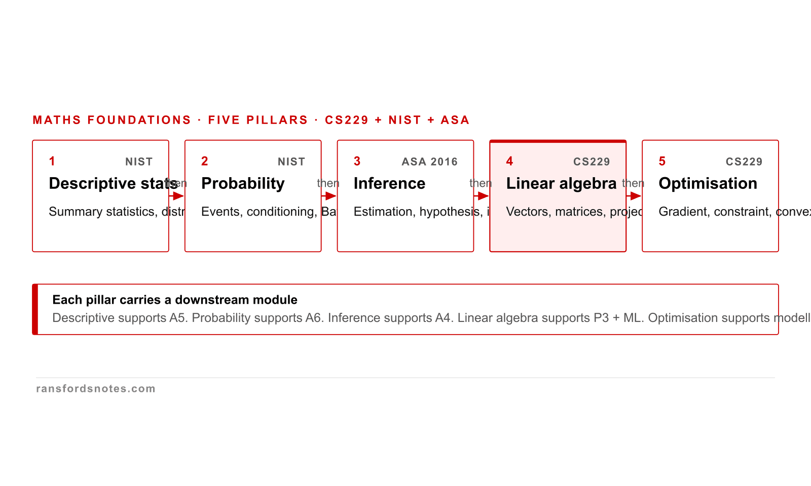
Five mathematical foundations and what each one carries
Five mathematical foundations carry the rest of the stage: descriptive statistics, probability, inference, linear algebra, optimisation.
Five foundations carry the rest of the stage: descriptive statistics, probability, inference, linear algebra, optimisation. Each binds to a downstream module; thinning any foundation breaks a downstream chapter. Stanford CS229 names the same five as prerequisites.
Four published languages for communicating uncertainty
Uncertainty has four published languages; mixing confidence with credible intervals is the most common reporting defect.
Uncertainty has four published languages: confidence interval (frequentist), credible interval (Bayesian), prediction interval (single new observation), tolerance interval (population coverage). Mixing them creates the most common reporting defect. NIST Engineering Statistics Handbook §1.3.5 defines all four.
Real-world application · 2006 onwards
Netflix Prize: $1 million for a 10% improvement in prediction accuracy
In 2006, Netflix offered a $1 million prize to the first team that could improve its film recommendation algorithm by 10%. The contest ran for three years, attracted 51,000 teams from 186 countries, and ultimately required the top entrants to form a grand ensemble of 107 different algorithms to claim the prize.
At the core of the winning solution was matrix factorisation: decomposing a sparse user-by-film ratings matrix into lower-dimensional vector representations for each user and each film. The dot product of a user vector and a film vector predicts the rating. Training the vectors required gradient descent to minimise prediction error across millions of examples.
The Netflix Prize made matrix factorisation the dominant recommendation technique for a decade. Every streaming service, e-commerce platform, and social feed now relies on variants of the same linear algebra. The mathematics this module covers is not academic preparation. It is the engine running in production at scale right now.
The winning team combined gradient boosted machines, neural networks, and matrix factorisation. What mathematical structures underpin each of those three methods?
Data practitioners who lack mathematical foundations can apply tools without understanding them. That gap causes failures at scale: a model that works in a notebook but fails in production, a recommendation system that amplifies bias, or a statistical test that produces false confidence. The goal here is not to make you a mathematician but to give you the mental models that let you read research papers, debug models, and evaluate vendor claims critically.
With the learning outcomes established, this module begins by examining vectors, matrices, and why they matter for data in depth.
21.1 Vectors, matrices, and why they matter for data
A vector is an ordered list of numbers: [3.2, 0.8, 1.5]. In data contexts, vectors represent things. A product in an e-commerce catalogue might be represented as a vector of feature values: [price, category_encoded, average_rating, days_since_launch]. A word in a language model is represented as a 768-dimensional or 1536-dimensional embedding vector where proximity in that high-dimensional space corresponds to semantic similarity.
A matrix is a rectangular array of numbers. A dataset with 10,000 rows and 15 features is a 10,000 by 15 matrix. Multiplying that matrix by a weight matrix transforms the features into a new representation. This operation, matrix multiplication, is the core computation of every neural network layer, every linear regression, and every principal component analysis.
The dot product of two vectors measures their similarity: it is the sum of element-wise products. If two user preference vectors point in the same direction in feature space, their dot product is large. If they are orthogonal (no shared preference), it is zero. This is why collaborative filtering works: users with similar preference vectors get similar recommendations.
Transposing a matrix (flipping rows and columns) is a constant operation in data processing: converting column vectors to row vectors, reshaping batches for neural network layers, and computing covariance matrices all use transposition. The covariance matrix of a dataset is computed as the product of the data matrix transposed with itself, divided by the number of observations minus one.
With an understanding of vectors, matrices, and why they matter for data in place, the discussion can now turn to gradient descent: training as optimisation, which builds directly on these foundations.
“Linear algebra is the mathematics of data. Data tables are matrices. Observations are vectors. Models are linear transformations. Understanding this makes every algorithm legible.”
Gilbert Strang, MIT OpenCourseWare 18.06: Linear Algebra
Strang's framing is useful for practitioners: linear algebra is not an abstract prerequisite but the direct description of what happens to data as it flows through a pipeline or a model.
21.2 Gradient descent: training as optimisation
Training a machine learning model means finding the parameter values that minimise a loss function: a number that measures how wrong the model's predictions are. Gradient descent is the algorithm that does this. The gradient of the loss with respect to each parameter tells you the direction of steepest increase. To minimise the loss, you move in the opposite direction, scaled by a learning rate.
Each update step is: parameter = parameter minus (learning rate times gradient). Repeat this millions of times across many examples and the model converges on parameters that produce low loss. The learning rate is the most consequential hyperparameter: too large and the model oscillates; too small and training takes impractically long or stalls in a local minimum.
Stochastic gradient descent (SGD) computes the gradient on a small random batch of examples rather than the full dataset. This introduces noise into the gradient estimate but reduces computation per step enormously. Mini-batch SGD with batch sizes of 32 to 256 is the standard in practice. Adaptive optimisers like Adam adjust the learning rate per parameter based on recent gradient history, which typically accelerates convergence.
Backpropagation is the algorithm that computes gradients efficiently in neural networks. It applies the chain rule of calculus to propagate error signals from the output layer backward through each layer, computing each layer's contribution to the loss. Without backpropagation, training deep networks would be computationally infeasible.
With an understanding of gradient descent: training as optimisation in place, the discussion can now turn to bayes' theorem and probabilistic reasoning, which builds directly on these foundations.
21.3 Bayes' theorem and probabilistic reasoning
Bayes' theorem states that the probability of a hypothesis given observed evidence equals the prior probability of the hypothesis multiplied by the likelihood of the evidence given the hypothesis, divided by the probability of the evidence. Written compactly: P(H|E) = P(E|H) x P(H) / P(E).
The power of Bayes is in updating beliefs as new evidence arrives. A spam filter has a prior belief about the probability of an email being spam. When it observes specific words (the evidence), it updates that belief. After seeing many words, the posterior probability is high enough to classify the email. This is Naive Bayes classification: it assumes features are conditionally independent given the class label (a simplification, but one that works well in practice for text).
Medical testing is the canonical illustration of Bayes. A test with 99% sensitivity and 99% specificity for a disease affecting 0.1% of the population will produce more false positives than true positives when applied to the general population. Specifically, of 1,000 people tested: 1 has the disease and tests positive (true positive), 0 has the disease and tests negative (false negative in 1% of cases), and approximately 10 healthy people also test positive (false positive rate of 1% applied to 999 healthy people). The positive predictive value is 1/11, or about 9%. Understanding base rates is essential for interpreting model outputs.
With an understanding of bayes' theorem and probabilistic reasoning in place, the discussion can now turn to information theory: entropy and signal, which builds directly on these foundations.
Common misconception
“A model with 99% accuracy on a test set is reliable for production.”
Accuracy is misleading for imbalanced datasets. A fraud detection model trained on data where 0.1% of transactions are fraudulent can achieve 99.9% accuracy by predicting 'not fraud' for every transaction. The correct metrics are precision (what fraction of flagged transactions are genuinely fraudulent), recall (what fraction of fraudulent transactions were caught), and F1 score or area under the ROC curve. Always examine the class distribution before interpreting accuracy figures. The base rate fallacy (ignoring prior probabilities) leads to this error.
21.4 Information theory: entropy and signal
Shannon entropy quantifies the average uncertainty in a probability distribution. A fair coin has maximum entropy (1 bit) because both outcomes are equally likely. A biased coin that lands heads 99% of the time has very low entropy because the outcome is almost entirely predictable. Entropy is the foundation of information theory, compression algorithms, decision trees, and the cross-entropy loss function used to train classification models.
Cross-entropy loss measures the difference between a model's predicted probability distribution and the true distribution (usually a one-hot vector where the correct class has probability 1 and all others have probability 0). Minimising cross-entropy during training pushes the model to assign high probability to correct predictions.
Mutual information measures how much knowing one variable reduces uncertainty about another. It is used in feature selection (high mutual information between a feature and the target means the feature is informative), in clustering evaluation, and in the information bottleneck method for training compressed representations in neural networks.
KL divergence (Kullback-Leibler divergence) measures how much one probability distribution differs from a reference distribution. It appears in variational autoencoders, in reinforcement learning policy optimisation, and in evaluating how well a fitted statistical distribution matches empirical data.
“The fundamental problem of communication is that of reproducing at one point either exactly or approximately a message selected at another point.”
Claude Shannon, 'A Mathematical Theory of Communication', Bell System Technical Journal (1948)
Shannon's 1948 paper founded information theory. His entropy formula H = -sum(p log p) has since appeared in machine learning loss functions, compression algorithms, cryptography, and biology. The concept of measuring information as uncertainty reduction is one of the most widely applied ideas in all of science and engineering.
A collaborative filtering system represents each user as a 64-dimensional embedding vector. User A has vector [0.8, 0.2, ...] and User B has vector [0.7, 0.3, ...]. User C has vector [-0.6, -0.1, ...]. Without computing exact values, which pair of users is most likely to receive similar recommendations, and why?
A diabetes screening test has 95% sensitivity and 90% specificity. The disease affects 2% of the population being screened. A patient tests positive. Which statement correctly estimates the probability that the patient actually has diabetes?
During training, a classification model's cross-entropy loss decreases from 2.3 to 0.1 over 50 epochs. What does this indicate about the model's probability assignments to the correct class?
Key takeaways
- Vectors represent data points and embeddings; matrices represent datasets and linear transformations. The dot product measures similarity and is the core operation in recommendation systems, attention mechanisms, and linear regression.
- Gradient descent is the universal optimisation algorithm for model training. It iteratively adjusts parameters in the direction that reduces the loss function, using gradients computed by backpropagation.
- Bayes' theorem updates beliefs given evidence. The base rate fallacy (ignoring prior probabilities) causes systematic misinterpretation of model outputs, especially in imbalanced classification tasks.
- Shannon entropy quantifies uncertainty. Cross-entropy loss minimises the difference between predicted and true probability distributions. Mutual information measures how much one variable reduces uncertainty about another.
Standards and sources cited in this module
Gilbert Strang, 'Introduction to Linear Algebra' (5th ed.)
The standard reference for linear algebra as applied to data. MIT OpenCourseWare 18.06 videos are freely available.
Claude Shannon, 'A Mathematical Theory of Communication' (1948)
Founding paper of information theory. Source of the entropy formula and the connection between probability and information.
Netflix Prize documentation (2006-2009)
Context for the application of matrix factorisation and gradient descent to recommendation at scale.
Christopher Bishop, 'Pattern Recognition and Machine Learning' (2006)
thorough treatment of Bayesian reasoning, information theory, and probabilistic graphical models as applied to data.
Kingma and Ba, 'Adam: A Method for Stochastic Optimization' (2014)
Source paper for the Adam optimiser. Explains adaptive learning rates and their advantages over standard SGD.
Module 21 of 26 · Practice & Strategy